The vector rotations of the plane (i.e. centred in the origin), are derived analytically (by coordinates) as linear applications of determinant \(1\), which makes it possible to characterise them integrally and to identify them with the points of the trigonometric circle, their composition corresponding to the complex multiplication.

1. Vector rotations of the plane

The notion of rotation in the Euclidean plane \(\mathbb R^2\) can be understood intuitively. A rotation is a “transformation” of the plane (a bijection from the plane onto itself) which makes its points “rotate” around a given fixed point, its centre. A rotation is said to be a vector rotation if its centre is the origin \(O=(0,0)\) of the plane. The understanding of rotations of the plane is based on the understanding of vectorial rotations, which we consider here.

1.1. Linear applications

The rigorous description of the concept of (vector) rotation is done through the notions of linear application and Euclidean norm. A linear application is a function \(f:\mathbb R^2\to \mathbb R^2\), which “preserves addition and multiplication by a constant on each coordinate”. In other words, if \((x,y),(u,v)\in\mathbb R^2\) are two vectors of the plane and \(a,b\in\mathbb R\) two real numbers, we require that \(f(a. (x,y)+b.(u,v))=a.f(x,y)+b.f(u,v)\) (recall that \((x,y)+(u,v)=(x+u,y+v)\) and that \(a.(x,y)=(a.x,a.y)\)). It can be shown that a linear application \(f:\mathbb R^2\to \mathbb R^2\) always has the form \(f(x,y)=(ax+by,cx+dy)\), for uniquely determined real numbers \(a,b,c,d\). The real number \(ad-bc\) is called the determinant of \(f\).

1.2. Norm and vector isometries

The (Euclidean) norm of a vector \((x,y)\in\mathbb R^2\) of the plane is the real number \(||(x,y)||=\sqrt{x^2+y^2}\). A (vector) isometry of the plane is a linear application \(f:\mathbb R^2\to \mathbb R^2\) which “preserves” the norm of the vectors. In other words, such an application has the following property: for any vector \((x,y)\in\mathbb R^2\), we have \(||f(x,y)||=||(x,y)||\). Returning to the previous description of a linear application \(f\) from coefficients \(a,b,c,d\), this is interpreted analytically (from the coordinates) as \(\sqrt{x^2+y^2}=\sqrt{(ax+by)^2+(cx+dy)^2}\).

1.3. Analytical definition of vector rotations

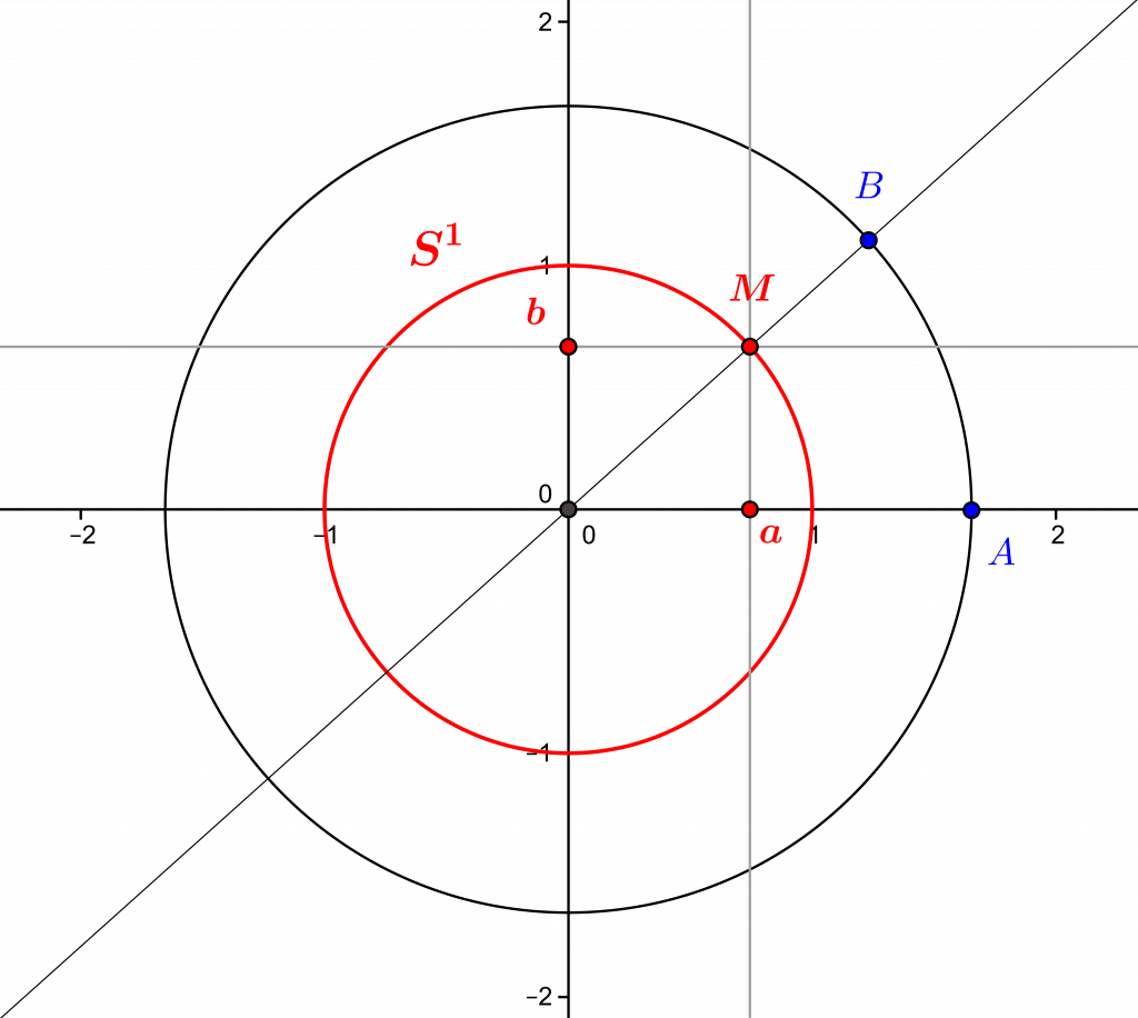
It can be shown that the determinant of a vector isometry of the plane can only be \(1\) or \(-1\), and a (vector) rotation of the plane is then by definition a vectorial isometry of determinant \(1\) (an isometry of determinant \(-1\) is an orthogonal symmetry with respect to a vectorial line). In this case, we also have \(a=d\) and \(b=-c\), and a rotation is then exactly an application \(f: \mathbb R^2\to \mathbb R^2\) of the form \(f(x,y)=(ax-by,bx+ay)\), with \(a,b\) two real numbers such that \(a^2+b^2=1\), i.e. such that the point \(a,b\) is on the trigonometric circle. In other words, there exists a bijection between the set of plane vectorial rotations and the trigonometric circle \(S^1\), which exchanges the rotation \(r\) described by \(r(x,y)=(ax-by,bx+ay)\) and the point \((a,b)\) of the circle \(S^1\).

2. Vector rotations and the trigonometric circle

2.1. The group of plane vector rotations

Using this approach, it can in fact also be shown that each vector rotation \(r\) defines a bijection from the Euclidean plane \(\mathbb R^2\) onto itself. It is enough for that to “invert” the following system of equations: \[\left\{\begin{array}{ll} ax-by = u\\bx+ay = v,\end{array}\right.\] where \((u,v)\) and \((x,y)\) are points of the plane linked by \((u,v)=r((x,y))\), if \(r(x,y)=(ax-by,bx+ay)\). In other words, the conditions on \(a\) and \(b\) which characterise a rotation allow to express \((x,y)\) as a function of \((u,v)\), in the form \((u,v)=(au+bv,-bu+av)\). Now, since this amounts to establishing that \(r\) is a bijection and describing its inverse bijection \(r^{-1}\), we see that the inverse of a rotation is itself a rotation, here \(r^{-1}(x,y)=(ax+by,-bx+ay)\).

Moreover, the composition of two rotations is itself a rotation. Indeed, if \(r(x,y)=(ax-by,bx+ay)\) and \(s(x,y)=(cx-dy,dx+cy)\) are two rotations, by applying \(r\) and then \(s\) we can describe the application \(s\circ r(x,y)\) as \(s(r(x,y))=s(ax-by,bx+ay)=((ca-db)x-(cb+ad)y,(cb+ad)x+(ca-db)y)\). It is then easy to calculate \((ca-db)^2+(cb+ad)^2=1\), so that \(s\circ r\) is indeed a rotation. Since the identical application \(Id:\mathbb R^2\to \mathbb R^2\) described by \(Id((x,y))=(x,y)\), which leaves the Euclidean plane invariant, is itself a rotation, we see that the set of vectorial rotations of the plane is a group for the operation of composition of the applications (in fact a subgroup of the group of the vectorial isometries). We note here \(\mathcal R\) this group of rotations.

2.2. Isomorphism between the groups \((\mathcal R,\circ)\) and \((S^1,\times)\)

We have mentioned the existence of a bijection between the set \(\mathcal R\) of vector rotations and the trigonometric circle \(S^1\), which exchanges the rotation \(r(x,y)=(ax-by,bx+ay)\) and the point \((a,b)\). Now, we can perform a multiplication operation between the points of the circle \(S^1\), based on complex multiplication (see What is a complex number ? – to appear). Indeed, the trigonometric circle is the set of complex numbers of modulus \(1\), so the multiplication of two points \(z,w\) of \(S^1\) is still a point of \(S^1\), since \(|z\times w|=|z|\times |w|=1\). Moreover, the inverse of \(z\) being \(\dfrac{\overline z}{|z|^2}=\overline z\) if \(z\in S^1\), the inverse of an element of \(S^1\) is also in \(S^1\), since $|z|=|\overline z|$.

In other words, the circle \(S^1\) is also a group for complex multiplication, and the bijection between \(\mathcal R\) and \(S^1\) “exchanges” these two group structures, by “transforming” the composition of rotations into the multiplication of the corresponding complex numbers. In other words, from an algebraic standpoint, the set \(\mathcal R\) of vectorial rotations and the trigonometric circle \(S^1\) are “essentially” the same mathematical object.

2.3. Rotations act on points of \(S^1\)

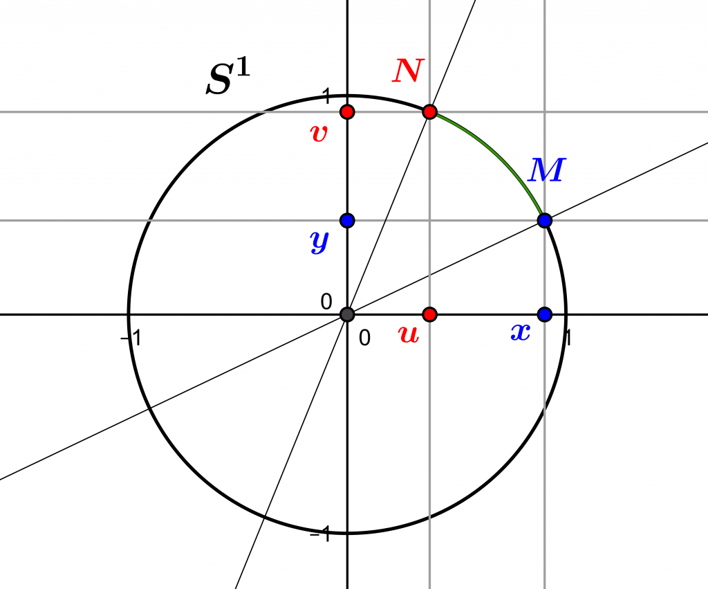
Another way of looking at their relationship is to consider that the vector rotations actually “act” on the points of the circle \(S^1\). Mathematically, this means that such a rotation transforms one point of this circle into another point of this circle. This is intuitively obvious: any rotation centred at the origin of the plane should “act” on points of the plane while maintaining their distance from the origin, since it is an isometry. Thanks to the analytical description given earlier, it is possible to say more: if \(M=(x,y)\) and \(N=(u,v)\) are two points of the trigonometric circle, there exists a unique rotation which sends \(M\) onto \(N\). To determine this one, one takes again the preceding system of equations, which one solves this time to identify \(a\) and \(b\). A unique solution is found, either \(a=-\dfrac v y,b=-\dfrac u y\) if \(x=0\) (i.e. if \(M=(0,1)\)), or \(a=xu+yv,b=xv-yu\) if \(x\neq 0\) (i.e. if \(M\neq (0,1)\)).

The analytical method – i.e. using coordinates – thus allows the vectorial rotations of the plane and their relation to the points of the trigonometric circle to be described in a transparent way.

3. Rotations and subfields of \(\mathbb R\)

3.1. Subfields of \(\mathbb R\)

A subfield of the set \(\mathbb R\) of real numbers is a subset \(K\) of \(\mathbb R\) which contains \(0\) and \(1\) and is “closed” for the operations \(+\) and \(\times\), as well as for the inversion of its non-zero elements. In other words, it is a subset \(K\) of \(\mathbb R\) verifying the following properties:
– \(0,1\in K\)
– if \(a,b\in K\), then \(a+b\in K\) and \(a.b\in K\)
– if \(a\in K\) and \(a\neq 0\), then \(1/a\in K\).

There exist many subfields of \(\mathbb R\) : the set \(\mathbb Q\) is an example, and one can easily show that any subfield of \(\mathbb R\) contains \(\mathbb Q\). The set noted \(\mathbb Q(\sqrt 2)\) of real numbers of the form \(a+b\sqrt 2\), with \(a,b\in\mathbb Q\) is another example. The set \(C\) of constructible numbers (with the ruler and the compass) is yet another example.

3.2. The affine plane associated with a subfield

If \(K\) is a subfield of \(\mathbb R\), then we can form the “affine plane” associated to \(K\): this is the set \(K^2=K\times K\), analogous to the Euclidean plane \(\mathbb R^2\) associated to \(\mathbb R\). The set \(K^2\) of pairs \((a,b)\) of elements of \(K\) is then a subset of the plane \(\mathbb R^2\). The fact that \(K\) is a subfield makes it possible to reproduce in \(K^2\) all affine geometry: one can speak about lines, equations of lines, study the intersection of two lines by solving the system formed by their equations, etc…

Affine geometry is essentially described in terms of points and linear algebra, i.e. the consideration of linear applications, such as those we introduced at the beginning of the article in the Euclidean plane. A linear application from \(K^2\) into \(K^2\) is therefore exactly the same as what we have defined for \(\mathbb R^2\). In this case it is also still possible to describe it as a function \(f:K^2\to K^2\) of the form \(f(x,y)=(ax+by,cx+dy)\), with \(a,b,c,d\in K\) this time.

3.3. Rotations in any plane

When we introduced rotations as linear applications, we defined them as vector isometries of determinant \(1\). Since an isometry is defined by preserving the Euclidean norm of the vectors, i.e. the real number \(\sqrt{x^2+y^2}\) for a vector \(x,y)\in R^2\), it may seem impossible to define an isometry of \(K^2\) in general. Indeed, in some subfields of K one cannot always extract a square root; this is the case for example of \(\mathbb Q(\sqrt 2)\), which contains \(3\) but not \(\sqrt 3\). However, it is enough to preserve the square of the norm to preserve the norm, so the definition does not pose a problem. But “analytically”, a rotation is a linear application \(f(x,y)=(ax-by,bx+ay)\) with \(a,b\in\mathbb R\) and \(a^2+b^2=1\). Without even considering the norm, this description means that everything we did previously remains valid in the plane \(K^2\)!

3.4. A purely algebraic theory

Of course, in this plane the “trigonometric circle” is the set \(S_K=\{(a,b)\in K^2 : a^2+b^2=1\}\), which is in general a subset of \(S^1\) that contains fewer points. But the identification of the group of vectorial rotations of \(K^2\) with \(S_K\) remains valid, as does the solution of the systems of equations presented here. This goes against the naive intuition that the theory of plane rotations is related to real trigonometric cosine and sine functions, and can therefore only be developed when such functions are available, which is not the case on the subfields of \(\mathbb R\) in general. In fact, this is a purely algebraic theory, and can be interpreted in the framework of Clifford algebras, a mathematical concept dear to physicists.